🔎 MACROS#

Inputs files#

The first step to make the macros work is to configure the input_file.txt. The first parameter that macros will require from the user is to select an input file:

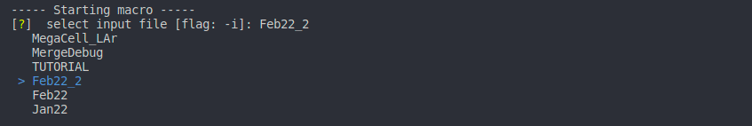
The formatting of this file need to be conserved to have read it correctly. Check io_functions.py->read_input_file(). You can turn debug=True when running the macros to check what is being loaded. You will see different sections:

DAQ INFO#

(In principle this section does not need to be changed.)

TYPE: ADC        # Acquisition system (ADC/OSC)
MODEL: 5725S     # Model used
BITS: 16384      # Dynamic range
DYNAMIC_RANGE: 2 # Dynamic range
SAMPLING: 4e-9   # Sampling: 4ns = 1 bin

RUNS INFO#

Here you configure the runs you are going to analyze depending on the data taking.

RAW_DATA: DAT                                 # Type of raw data you are using (DAT/ROOT)
RAW_PATH: data/BASIC/raw                      # Path to the data
NPY_PATH: data/BASIC/${USER}/npy              # Path to the npz outputs
OUT_PATH: data/BASIC/${USER}                  # Path to the analysis outputs

OV_LABEL: OV1,OV2                             # Labels for the different OV runs
CALIB_RUNS: 01,08                             # Calibration runs: trigger+light with pulse generator; laser to single photo electron (SPE) level
LIGHT_RUNS: 09                                # Light runs: trigger+light with pulse generator; laser with more intensity
NOISE_RUNS: 17,128                            # Noise runs: laser OFF + trigger pulse generator, "random trigger".
ALPHA_RUNS: 25                                # Alpha runs: coincidence trigger 2SiPMs; LAr scintillation light with alpha deposition
MUONS_RUNS: 29                                # Muons runs: coincidence trigger 2SiPMs;  LAr scintillation light with muon deposition
CHAN_LABEL: SiPM0,SC                          # Labels for the different channels
CHAN_TOTAL: 0,6                               # ADC channels (wave0.dat, wave6.dat stored raw files)
CHAN_POLAR: -1,1                              # Polarity of the channels (RawADC in SiPMs are negative in this setup)
CHAN_AMPLI: 250,1300                          # Amplification factor for each channel

BRANCH INFO#

In this section the presets for loading/saving *.npz files are configured. In principle, you don’t need to change this but check in io_functions.py -> get_preset_list() for more info.

#PRESETS USED: 0,  1,  2,  3,  4,  5,  6
LOAD_PRESET: NON,RAW,ANA,ANA,EVA,EVA,ANA
SAVE_PRESET: NON,ALL,EVA,CAL,CAL,NON,DEC

ANA DEFAULTS#

PED_KEY: PreTriggerMean # Key to be used for the pedestal

CHARGE INFO#

Here you define integration ranges to get the charge of your signal. There are different calibration modes check wvf_functions.py -> integrate_wvfs() for more info.

TYPE: ChargeAveRange,ChargePedRange,ChargeRange # Integration type (ChargeAveRange,ChargeRange*,ChargePedRange*)
REF: AveWvf                                     # Reference average waveform to compute the integration ranges (AveWvf,AveWvfSPE)
I_RANGE: 0.1,0.5,0.5,0.5,0.5                    # Initial integration time (in us) -> ChargeRange0_ini = peak-0.1us
F_RANGE: 0.1,0.5,1.0,2.0,4.0                    # Final integration time (in us)   -> ChargeRange0_end = peak+0.1us

CUTS INFO#

If you need to remove some events to perform the analysis you can include some cuts in this section. You can add as many cuts as needed by adding a number to the key (0CUT,1CUT,2CUT…).

0CUT_CHAN: 0,6          # Channels to apply the cut
0CUT_TYPE: cut_df       # Type of cut
0CUT_KEYS: AnaValleyAmp # Keys to apply the cut
0CUT_LOGIC: bigger_than # Logic of the cut
0CUT_VALUE: 0           # Value of the cut (AnaValleyAmp>0 are the events that we want to keep)
0CUT_INCLUSIVE: False   # Inclusive cut (False event need to be in all the channels)

Flags#

You can start by running the macros in the guide mode, and it will ask you for the input variables needed (see an example for the input file)

Once you are sure about the variables to use you can run the macro with the defined flags:

-h or --help
-i or --input_file
-l or --load_preset
-s or --save_preset
-k or --key
-v or --variables
-r or --runs
-c or --channels
-f or --filter
-d or --debug

They may be useful when you do not need to run a macro over all the runs or channels configured in the input file. For example, if you want to run the macro 00Raw2Np.py only for the runs 1 and 2 and channels 0 and 1 you can run:

python3 00Raw2Np.py -r 1,2 -c 0,1

Analysis Macros#

You will see that the macros start with the same of these common lines:

import sys; sys.path.insert(0, '../'); from lib import *
default_dict = {"runs":["CALIB_RUNS","LIGHT_RUNS","ALPHA_RUNS","MUONS_RUNS","NOISE_RUNS"],"channels":["CHAN_TOTAL"],"key":["ANA_KEY"]}
user_input = initialize_macro("00Raw2Np",["input_file","debug"],default_dict=default_dict, debug=True)
info = read_input_file(user_input["input_file"][0], debug=user_input["debug"])

which imports all the functions of the library (from lib folder) to be used and define the default values that each macro need to work. Also, the user input is initialized with the initialize_macro function. The first argument is the name of the macro, the second is the list of arguments that the macro needs to work, and the third is the default values for the arguments.

00Raw2Np#

This macro converts the raw files, usually *.dat, from RAW_PATH into .npz files at NPY_PATH. It is using the binary2npy() function. Notice that once you run this macro you will have new folders npy/runXX/chYY where the *.npz files are stored.

binary2npy(np.asarray(user_input["runs"]).astype(str),np.asarray(user_input["channels"]).astype(str),info=info,compressed=True,force=True)

⏩ RUN (in macros folder) ⏩

python3 00Raw2Np.py

✅ If everything is OK you should get new folders /npy/runXX/chYY

where we see the destination file and if the different files existed previously, are overwritten etc…

01PreProcess #

This macro will process the {RawPedestal, RawPeak} variables for the RawADC that are computed and saved in .npz files. You will see as terminal output the saved files. By default, the saving is set to force = True and so if you pre-process files that already existed they will be overwritten.

for run, ch in product(np.asarray(user_input["runs"]).astype(str),np.asarray(user_input["channels"]).astype(str)):
    my_runs = load_npy([run],[ch], info, preset=info["LOAD_PRESET"][1], compressed=True, debug=user_input["debug"])
    
    compute_peak_variables(my_runs, key=user_input["key"][0], label="", debug=user_input["debug"])
    compute_pedestal_variables(my_runs, key=user_input["key"][0], label="", debug=user_input["debug"]) # Checking the best window in the pretrigger

    delete_keys(my_runs,[user_input["key"][0]]) # Delete previous peak and pedestal variables
    save_proccesed_variables(my_runs, info, preset=info["SAVE_PRESET"][1], force=True, debug=user_input["debug"])
    
    del my_runs
    gc.collect()

⏩ RUN (in macros folder) ⏩

python3 01PreProcess.py

02AnaProcesss #

This macro will process the {Pedestal, Peak} variables for the ADC are computed and saved in .npz files. You will see as terminal output the saved files. By default, the saving is set to force = True and so if you pre-process files that already existed they will be overwritten. However, we delete the RawKeys from the my_runs dictionary to save computing time (RawInfo don’t change).

for run, ch in product(np.asarray(user_input["runs"]).astype(str),np.asarray(user_input["channels"]).astype(str)):
    my_runs = load_npy([run],[ch], info, preset=info["LOAD_PRESET"][2], compressed=True, debug=user_input["debug"])
    compute_ana_wvfs(my_runs,debug=False)
    delete_keys(my_runs,['RawADC','RawPeakAmp', 'RawPeakTime', 'RawPedSTD', 'RawPedMean', 'RawPedMax', 'RawPedMin', 'RawPedLim']) # Delete branches to avoid overwritting

    compute_peak_variables(my_runs, label="Ana", key="AnaADC", debug=user_input["debug"])     # Compute new peak variables
    compute_pedestal_variables(my_runs, label="Ana", key="AnaADC", debug=user_input["debug"]) # Compute new ped variables using sliding window

    save_proccesed_variables(my_runs,preset=str(info["SAVE_PRESET"][2]),info=info, force=True)
    del my_runs
    gc.collect()

⏩ RUN (in macros folder) ⏩

python3 02AnaProcess.py

03Integration #

In this macro we compute the charge (example: integrate_wvfs(my_runs, ["ChargeAveRange"], "AveWvf", ["DAQ", 250], [0,100]))

 for run, ch in product(np.asarray(user_input["runs"]).astype(str),np.asarray(user_input["channels"]).astype(str)):
    my_runs = load_npy([run],[ch], info, preset=info["LOAD_PRESET"][3], compressed=True, debug=user_input["debug"])
    
    integrate_wvfs(my_runs, info=info, key=user_input["key"][0], debug=user_input["debug"])

    delete_keys(my_runs,user_input["key"])
    save_proccesed_variables(my_runs, preset=str(info["SAVE_PRESET"][3]),info=info, force=True, debug=user_input["debug"])
    del my_runs
    gc.collect()

It will be used for calibrating the sensors in the following macro.

⏩ RUN (in macros folder) ⏩

python3 03Integration.py

04Calibration #

Compute a calibration histogram where the peaks for the PED/1PE/2PE… are fitted to obtain the gain.

 for run, ch in product(np.asarray(user_input["runs"]).astype(str),np.asarray(user_input["channels"]).astype(str)):
    my_runs = load_npy([run],[ch], info, preset=info["LOAD_PRESET"][4], compressed=True, debug=user_input["debug"])

    label, my_runs = cut_selector(my_runs, user_input)
    popt, pcov, perr = calibrate(my_runs,[user_input["variables"][0]],OPT, debug=user_input["debug"])
    calibration_txt(run, ch, popt, pcov, filename="gain", info=info, debug=user_input["debug"])

The parameters are computed from the best fit parameters and covariance matrix obtained from the curve_fit function. These parameters are saved in a txt for each channel.

With the cuts functions we also compute the SPE waveform (that can be visualized with the Vis macros)

⏩ RUN (in macros folder) ⏩

python3 04Calibration.py

If everything is working as it should you should obtain the following plots:

Note that we perform two fits here, one for obtain the SPE gain and another to get the cross–talk through Vinogradov method. To go from one plot to the next one just type any keyword in the plot window. All the plots are saved in images folder and the fit parameters if you choose to save them in the analysis one. ✅

05Charge #

    ## Visualize average waveforms by runs/channels ##
    my_runs = load_npy(runs.astype(str),channels.astype(str),branch_list=["Label","Sampling","AveWvf"],info=info,compressed=True) #Remember to LOAD your wvf
    vis_compare_wvf(my_runs, ["AveWvf"], compare="RUNS", OPT=OPT)

    for run, ch in product(runs.astype(str),channels.astype(str)):
        my_runs = load_npy([run],[ch], branch_list=["ADC","TimeStamp","Sampling","ChargeAveRange", "NEventsChargeAveRange","AveWvf"], info=info,compressed=True)  #preset="ANA"
        print_keys(my_runs)

        ## Integrated charge (scintillation runs) ##
        print("Run ", run, "Channel ", ch)

        popt_ch = []; pcov_ch = []; perr_ch = []; popt_nevt = []; pcov_nevt = []; perr_nevt = []
        popt, pcov, perr = charge_fit(my_runs, int_key, OPT); popt_ch.append(popt); pcov_ch.append(pcov); perr_ch.append(perr)
        
        scintillation_txt(run, ch, popt_ch, pcov_ch, filename="pC", info=info) ## Charge parameters = mu,height,sigma,nevents ## 

⏩ RUN (in macros folder) ⏩

python3 05Charge.py

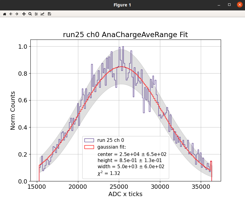
If everything is working as it should you should obtain the following histograms (raw and fitted) and a txt file with the scintillation parameters (if confirmed when asked through terminal) ✅

06Deconvolution #

🚧 … updating … 🚧

Before running the deconvolution macro make sure you have a clean laser/led signal that can be used as a template. The macro will load the alpha runs and rescale the light signal to the SPE amplitude according to AveWvfSPE calculated at calibration stage. Make sure you understand which type of runs you are using and run these scripts:

python3 11AverageSPE.py

python3 12GenerateSER.py

The deconvolution macro will:

Firstly, the average wvfs are deconvolved. From these the gauss filter cut-off (from the wiener filter fit) is extracted and saved.
Secondly, the previous calculated gauss filter is applied to deconvolve the ADC wvfs.
Finally, the deconvolved wvfs are saved for further process using the standard workflow.

for idx, run in enumerate(raw_runs):
    for jdx, ch in enumerate(ana_ch):
        my_runs = load_npy([run],[ch],preset=str(info["LOAD_PRESET"][6]),info=info,compressed=True)  # Select runs to be deconvolved (tipichaly alpha)     

        if "SiPM" in str(my_runs[run][ch]["Label"]):
            light_runs =  load_npy([dec_runs[SiPM_OV]],[ch],preset="EVA",info=info,compressed=True) # Select runs to serve as dec template (tipichaly light)    
            single_runs = load_npy([ref_runs[SiPM_OV]],[ch],preset="EVA",info=info,compressed=True) # Select runs to serve as dec template scaling (tipichaly SPE)   
        elif "SC" in str(my_runs[run][ch]["Label"]):
            light_runs =  load_npy([dec_runs[idx]],[ch],preset="EVA",info=info,compressed=True) # Select runs to serve as dec template (tipichaly light)    
            single_runs = load_npy([ref_runs[idx]],[ch],preset="EVA",info=info,compressed=True) # Select runs to serve as dec template scaling (tipichaly SPE)
        else:
            print("UNKNOWN DETECTOR LABEL!")
        
        keys = ["AveWvf","SER","AveWvf"] # keys contains the 3 labels required for deconvolution keys[0] = raw, keys[1] = det_response and keys[2] = deconvolution 

        generate_SER(my_runs, light_runs, single_runs)

        OPT = {
            "NOISE_AMP": 1,
            "FIX_EXP":True,
            "LOGY":True,
            "NORM":False,
            "FOCUS":False,
            "SHOW": True,
            "SHOW_F_SIGNAL":True,
            "SHOW_F_GSIGNAL":True,
            "SHOW_F_DET_RESPONSE":True,
            "SHOW_F_GAUSS":True,
            "SHOW_F_WIENER":True,
            "SHOW_F_DEC":True,
            "WIENER_BUFFER": 800,
            "THRLD": 1e-4,
            }

        deconvolve(my_runs,keys=keys,OPT=OPT)

        OPT = {
            "SHOW": False,
            "FIXED_CUTOFF": True
            }

        keys[0] = "ADC"
        keys[2] = "ADC"
        deconvolve(my_runs,keys=keys,OPT=OPT)

        save_proccesed_variables(my_runs,preset=str(info["SAVE_PRESET"][6]),info=info,force=True)
        del my_runs,light_runs,single_runs

generate_input_file(input_file,info,label="Gauss")

⏩ RUN (in macros folder) ⏩

python3 06Deconvolution.py

Visualizing Macros#

All the visualizing macros use the VisConfig.txt stored in the macros folder. This file contains the default values for the visualization. You can change the values in the file or when running the macro (it will show you the loaded values and ask the user if need to change a line).

MICRO_SEC: True            # True if you want to see the time in microseconds
PE: True                   # True if you want to see the charge in PE (requres calibration.yml file --> saved to the data/analysis folder) 
NORM: False                # True if you want to normalize the waveforms
LOGX: False                # True if you want to see the x axis in log scale
LOGY: False                # True if you want to see the y axis in log scale
LOGZ: False                # True if you want to see the z axis in log scale
CHARGE_KEY: ChargeAveRange # Key to be used for the charge 
PEAK_FINDER: False         #
CUTTED_WVF: 0              # To show all the events (-1), the cutted (0) or the uncutted (1)
LEGEND: False              # True if you want to see the legend
THRESHOLD: 1               # NORMALIZED Threshold for the peak finder (calibration fit)
WIDTH: 15                  # NORMALIZED Width for the peak finder (calibration fit)
PROMINENCE: 0.4            # NORMALIZED Prominence for the peak finder (calibration fit)
ACCURACY: 1000             # NORMALIZED Accuracy for the peak finder (calibration fit)
SHOW_AVE: AveWvf           # Average waveform to be shown if computed (AveWvf,AveWvfSPE,...)
SHOW_PARAM: True           # True if you want to see the parameters of the fit
SHOW: True                 # True if you want to see the plot
COMPARE: NONE              # Comparissons in the same plot (NONE, RUNS, CHANNELS)
TERMINAL_MODE: True        # True if you want to see the plot in the terminal
PRINT_KEYS: False          # True if you want to print the keys of the dictionary
SCINT_FIT: True            # True if you want to fit the scintillation peaks

0XVisEvent #

We can visualize the individual events from the moment we pre-process the waveforms and obtain RawInfo.

my_runs = load_npy(np.asarray(user_input["runs"]).astype(str),np.asarray(user_input["channels"]).astype(str),preset=user_input["preset_load"][0],info=info,compressed=True) # preset could be RAW or ANA
label, my_runs = cut_selector(my_runs, user_input, debug=user_input["debug"])
vis_npy(my_runs, user_input["key"],OPT=OPT) # Remember to change key accordingly (ADC or RawADC)

⏩ RUN (in macros folder) ⏩

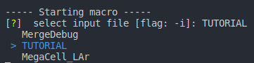
python3 0XVisEvent.py -r 1 -c 0,6
[?] select input file  [flag: -i]: TUTORIAL
[?] select load_preset [flag: -l]: ANA    (or RAW)
[?] select key         [flag: -k]: AnaADC (or RawADC)

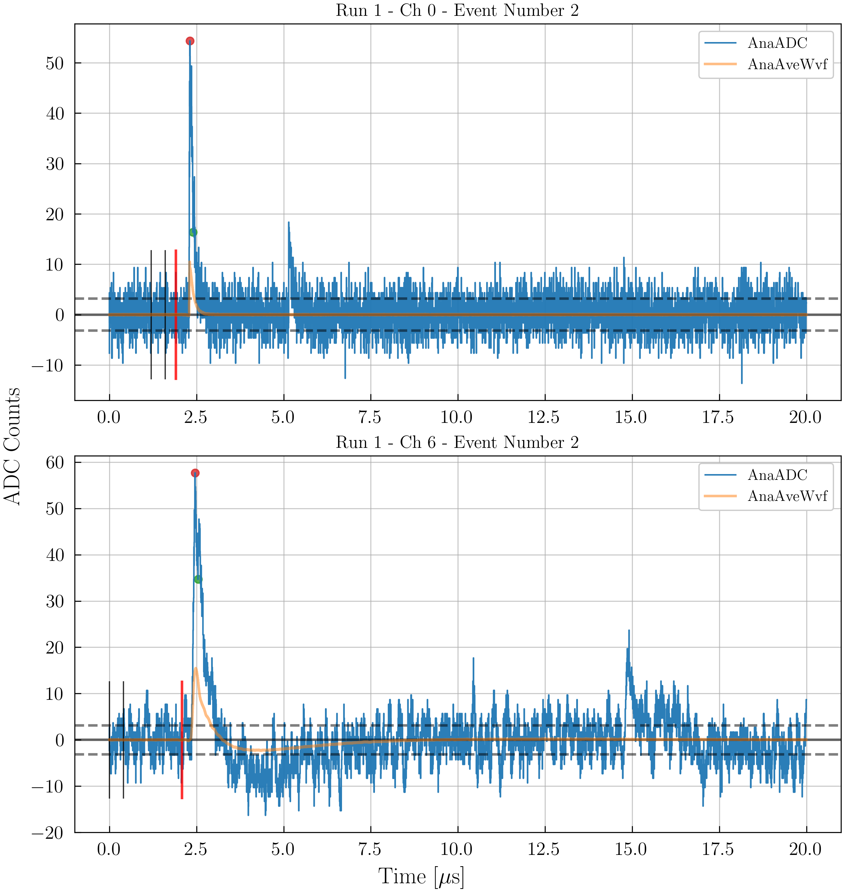
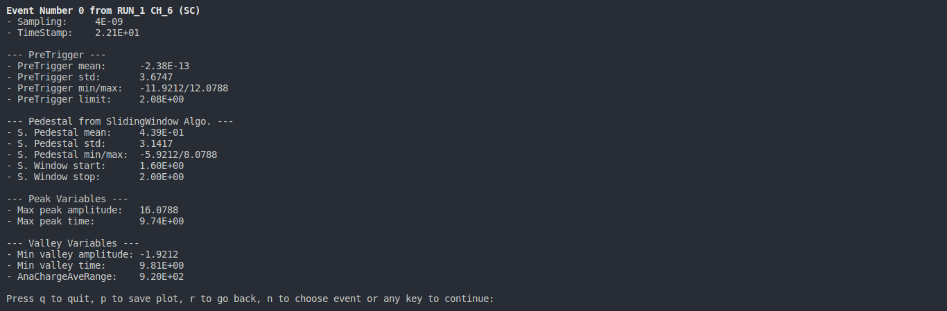
The individual events of different channels can be visualized together and with AveWvf superposed.

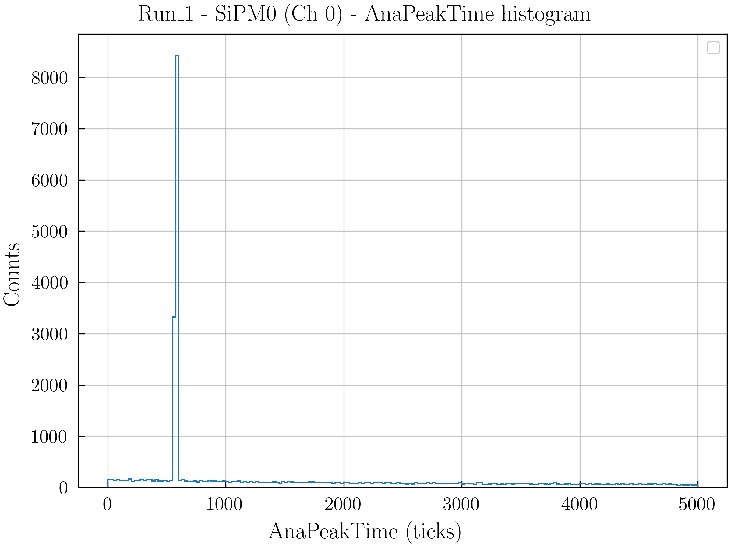
0YVisHist1D #

my_runs = load_npy(np.asarray(user_input["runs"]).astype(str), np.asarray(user_input["channels"]).astype(str), preset="EVA", info=info, compressed=True) # preset could be RAW or ANA
label, my_runs = cut_selector(my_runs, user_input, debug=user_input["debug"])
vis_var_hist(my_runs, user_input["variables"], percentile = [0.1, 99.9], OPT = OPT, select_range=False, debug=user_input["debug"])

⏩ RUN (in macros folder) ⏩

python3 0YVisHist1D.py -r 1 -c 0,6
[?] select input file  [flag: -i]: TUTORIAL
[?] select variables   [flag: -v]: AnaPeakTime (or the key we want to plot that is already computed)

0ZVisHist2D #

my_runs = load_npy(np.asarray(user_input["runs"]).astype(str), np.asarray(user_input["channels"]).astype(str), preset="EVA",info=info,compressed=True) # preset could be RAW or ANA
label, my_runs = cut_selector(my_runs, user_input, debug=user_input["debug"])
vis_two_var_hist(my_runs, user_input["variables"], OPT = OPT, percentile=[0.1,99.9], select_range=False)

⏩ RUN (in macros folder) ⏩

python3 0ZVisHist2D.py -r 1 -c 0,6
[?] select input file  [flag: -i]: TUTORIAL
[?] select variables   [flag: -v]: AnaPeakAmp,AnaChargeAveRange (or the key we want to plot that is already computed)

0WVisWvf#

my_runs = load_npy(np.asarray(user_input["runs"]).astype(str),np.asarray(user_input["channels"]).astype(str), info, preset=user_input["preset_load"][0], compressed=True, debug=user_input["debug"])
vis_compare_wvf(my_runs, user_input["variables"], OPT=OPT)

⏩ RUN (in macros folder) ⏩

python3 0WVisWvf.py -r 1 -c 0,6
[?] select input file  [flag: -i]: TUTORIAL
[?] select variables   [flag: -v]: AnaPeakAmp,AnaChargeAveRange (or the key we want to plot that is already computed)

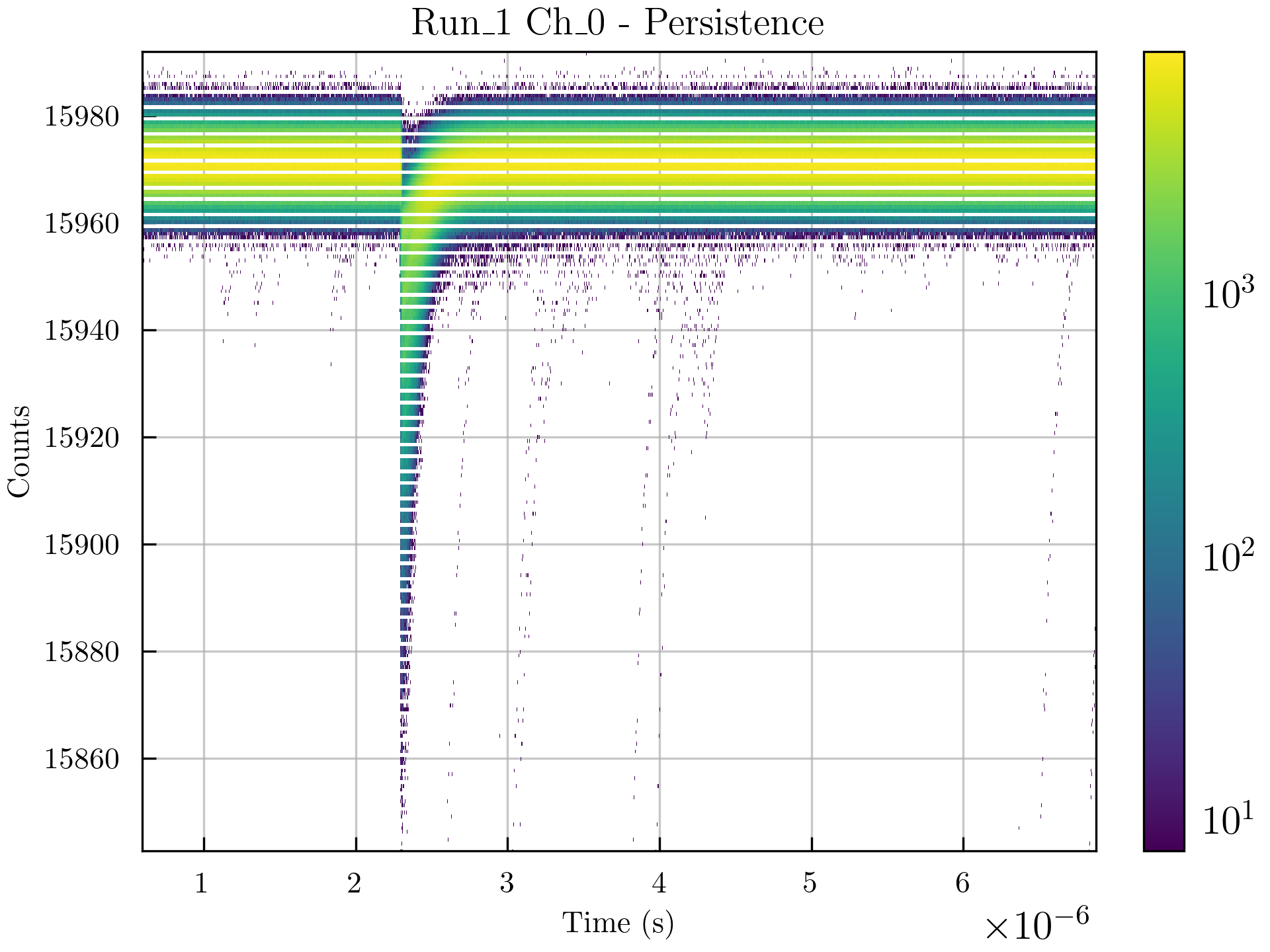
0VVisPersistence#

my_runs = load_npy(np.asarray(user_input["runs"]).astype(str),np.asarray(user_input["channels"]).astype(str), info, preset=user_input["preset_load"][0], compressed=True, debug=user_input["debug"])
vis_persistence(my_runs)

⏩ RUN (in macros folder) ⏩

python3 0VVisPersistence.py -r 1 -c 0
[?] select input file   [flag: -i]: TUTORIAL
[?]  select load_preset [flag: -l]: ANA

## We recomend to cut some events to see the persistence ##
[?] Select channels for applying **cut_df**: 0
[?] Select key for applying **cut_df**: AnaValleyAmp
[?] Select logic for applying **cut_df**: bigger
[?] Select value for applying **cut_df**: 0
[?] Select inclusive for applying **cut_df**: False

SCINT DOCUMENTATION

🔎 MACROS

Contents

🔎 MACROS#

Inputs files#

DAQ INFO#

RUNS INFO#

BRANCH INFO#

ANA DEFAULTS#

CHARGE INFO#

CUTS INFO#

Flags#

Analysis Macros#

00Raw2Np#

01PreProcess #

02AnaProcesss #

03Integration #

04Calibration #

05Charge #

06Deconvolution #

Visualizing Macros#

0XVisEvent #

0YVisHist1D #

0ZVisHist2D #

0WVisWvf#

0VVisPersistence#